Pivot Transformation in SSIS 2012 – Part 1 of 5

This article has been divided to five parts:

Part 1 – Getting data from flat file (Extract) – you are here

Part 2 – Sorting data (Transform).

Part 3 – Pivoting data (Transform).

Part 4 – Loading data to an SQL Server database table (Load).

Part 5 – Finalizing and Executing SSIS Package.

Abstract

Although, I found many ETL tutorials on the web which include Pivot transformations in SSIS, some of them were done using older versions of SSIS so they are out-of-date and others were not clear enough. That’s why I decided to create and share my own tutorial with detailed instruction on how to create ETL processes with Pivot transformation in SQL Server Integration Services 2012 (SSIS 2012).

Part 1

Introduction

If you are familiar with PIVOT keyword use in Transact-SQL or some other RDBMS which supports it, understanding Pivot transformation in SSIS will be a piece of cake. If not, no worries as I will explain everything here.

To make this example closer to what you might be dealing with at your daily job as an ETL Developer or Data Analyst, notice that I made this data:

• Without sorting any of the columns.
• has missing values, even though it is not obvious now, but the Pivot transformation will make it so because not we don’t have data for all states over all the months present in the dataset.

However, you may also want to know that the data used here is not real and I made it tiny on purpose for easier demonstration of the concept of Pivot in SSIS.

Problem

As many other ETL processes that you might deal with, we need to extract some data, transform it (with a Pivot transformation) and load it into SQL Server database’s table.

When to use Pivot?

It happens that you have a dataset and you find it necessary to change a column values into many new columns based on that column’s values, this is exactly where the Pivot transformation is of great help to you. Consider this example:

You have this dataset, and you want to convert it to something like this:

The months have been converted to Month Names and from values in “EventMonth” to many new columns within the process. If that’s what you want to achieve using SSIS, then this article is just made for you.

Solution

I will suppose that you know how to create a new SSIS project in Visual Studio, and how to create a new package, so either create a new SSIS project or download it from my GitHub, then you can follow these instructions:

Step 1

Add a new Flat File Connection by right-clicking the Connection Manager pane below your Data Flow designer and choose “New Flat File Connections…”

The dataset you will use in this tutorial is in the file “Aviation.tsv”, a tab-separated values file and you can find it on my GitHub. So after you download it, click “Browse” and select it from your local disk drive:

You better check the Preview page to make sure the columns are read correctly.

Name the connection manager “FF_Aviation” as shown above.

Step 2

In Control Flow tab of your package designer, add a new Data Flow Task from SSIS Toolbox and rename it to “DFT_Aviation”

Notice the annotation in the package I created, it is always a best-practice to write an annotation so when you get back to this package after a while or someone else tries to work on your package, you or they know what this package does, when and who created it.

Step 3

Double-click on the new Data Flow Task, so we navigate to the Data Flow tab to edit the flow of this task. Now your Data Flow tab should look like this:

I know! It is still empty but soon we will be adding elements as we go.

Step 4

Add a new Source Assistant from SSIS Toolbox, a dialog box will open automatically asking you for the Connection Manager to use with this Source Assistant, select Flat File under “Select source type” and you must find the Connection Manager you created in Step #1 with the name “FF_Aviation”, choose it and click OK.

Step 5

Rename the Source Assistant you created in the previous step to “FF_SRC_Aviation”.

Continue to the next part of this article – Sorting data (Transform).

Top 20 Unisex Names vs. Gender

Hello, in this post, I present a chart to show the distribution of names over genders for the top 20 unisex names which were the butter of my recent data analysis use case. The analysis was explained thoroughly and supplied with code snippets for those who want to apply it themselves using the lovely and efficient Python.

For more information about the data set of the original data analysis you can review the Data section in my previous blogpost.

These are the top 20 unisex names presented with the percentage of girls vs. boys.

Unisex Names vs. Gender (Click to enlarge)

If you have a story (a pleasant one hopefully) to share about one or more of these names, I would be glad to hear it in the comments below.

You can subscribe to this blog on the right and I would be very grateful if you share it on Twitter, Facebook or your favorite social network.

Top 20 Unisex Names – Data Analysis Use Case

Introduction

I’ve seen many websites like this one or that one talking about the most common unisex names or how to choose a cool unisex name for your baby, but I don’t know those so-called unisex names are based on what criteria and the authors there don’t say how they got them in the first place. In this article, I present a systematic way to get unisex names based on historical data of used baby names as far back as the year 1880. This article you are reading will go into the detailed analysis process, if you are not interested or you don’t care about the how-to, you can just jump to the results in Top 20 Unisex Names vs. Gender as I show the final unisex names with their distribution over both genders.

How do we define a unisex name?

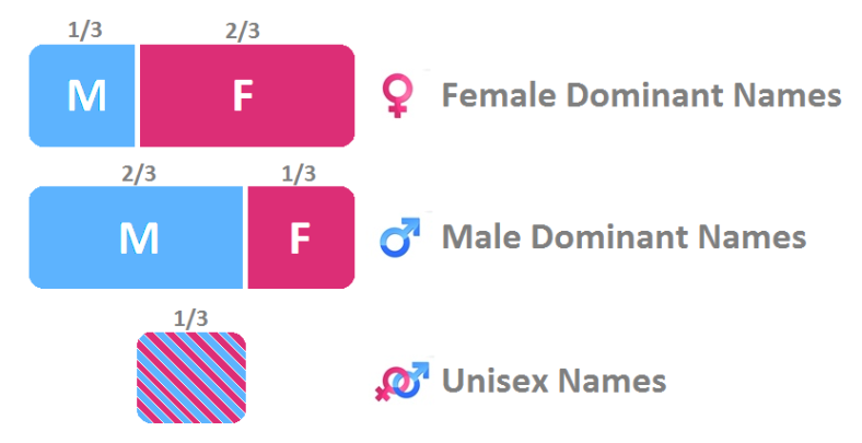
If I ask you what makes a name “unisex”, you might say, “Unisex names are those which can be used on a boy or a girl” or “those which I would not be at all surprised whether I hear they’re being used for a boy or a girl”. Here we see the second definition to be a subjective one because an unusual name for some gender might surprise you but could be very natural and even cool for the same gender, for someone else. So we revert back to the first definition but if a name is mostly used for a girl and very rarely used for a boy, will we consider that a unisex name? I don’t support that idea, we need some measure of commonality of the name over both genders. Why not we consult data of baby names? This is something historical and it is an objective measure as it represents the collective view of people to different names. The prevalence of some gender over some name should negate that name’s “unisex” flag. Let’s say we define the middle third (33.3%-66.6%) as our threshold, so if a name is used on, let’s say girls, more than two thirds, we call the name female-dominant. If it is used on less than one third, then we call that name “male-dominant” name. Otherwise, we are left with the middle third which I propose to consider “unisex” names. I will get back to this point in the Analysis section.

Tools Used for This Analysis

In this data analysis I will use:

Python v2.7.
Numpy v1.9.2.
Pandas v0.16.2, and
Matplotlib v1.4.2.

Python and its companion libraries comprise a handy and flexible tool for data analysis. That makes you focus on researching/investigating the use case instead of getting lost in the technical details of programming.

Data

The data I will use for this analysis is published by the United States Social Security Administration. The data cover the historical period between 1880 and 2010. The total names count under this dataset is approximately 322 million (exactly 322,402,727) names. For privacy considerations, a particular name must have at least 5 occurrences to be included in the data.

Understanding Data

Let’s take a closer look at the data, we have 131 plain text files (one for each year from the year 1880 to the year 2010). Each file contains unique (name-sex) records with the corresponding number of births of that name for that gender. That means you could find the name to be duplicated (or not, as some names are truly gender-specific). If you check the raw structure of the files, they are actually CSV (comma-separated values) files and that’s how we will read them into our Python Pandas data structures.

Few points worth mentioning about the data:

• If a name doesn’t exist in some year (file), it doesn’t exist as a record in that year’s file (You never find a name lingering there with 0 births!).
• If a name exists in some year (file) for one gender only (for example, Female), you will not find that name duplicated for Male with 0 births.
• As I mentioned earlier, the original data for this application is significantly big (almost 323 million baby names), but the data we have are not the individual records of births, instead, it is the births aggregated based on name-sex-year groups.
• The data doesn’t consider people who changed their names. Instead, it reports the name upon baby’s birth date only.

Analysis

As I mentioned above, I consider the names which are distributed over both genders with one gender percentage within the range from 33.3% to 66.6% as unisex names, so now we need a way to make some data slicing and dicing to get to those names. Try to think about or even write down a few steps to make it before you read on as I am about to spoil it 🙂

So what we need is to get the sweet spot in blue-purple (check the figure below). We need to make a group of all names by name (regardless of the year) and sum its births (for M male/F female from the Sex column). Notice that this analysis is not covering a specific year or decade. Instead, it takes the whole history of names and as far back as we have data  (the year 1880).

Here is my approach to get unisex names:

1. Put names (name-sex-year-births) in a dataframe.
2. Group the dataframe in Step #1 by name.
3. Exclude those names with records less than 50 (as we want common names only, if we didn’t make this Step, we could get a name which came up in one year only as 5 girls and 4 boys as a unisex name!)
4. Pivot the resultant dataframe to convert the values of Sex column (F, M) into columns and aggregate the births bases on the Sex value.
5. Copy the (F, M) columns from the dataframe in the Step #4 into a new dataframe.
6. Normalize them there to have the proportion of both genders.
7. Add the normalized (F, M) columns to the dataframe you got in Step #4 as new columns (Fprop, Mprop).
8. Add a new column total_births, it will hold the sum of the columns (F, M) for every row in the dataframe.
9. Exclude those rows with less than 8000 births.
10. Subset the DataFrame in Step #9, the criteria for subsetting is applied on rows and it only accepts a row if the proportion of female is between 0.3333 and 0.6666.

As we go through the Steps below, I will keep reminding you where we are.

This python code will take care of Step #1 for us:

# library imports
import numpy as np
import pandas as pd

# initialize variables
all_names = None # main dataframe
names_year_list = [] # empty list

# the years range in the data
years_range = range(1880, 2011)

# a list of the headers of the dataframe we are about to build
cols = ['name', 'sex', 'births']

# loop through the files
for year in years_range:

# file path
file_path = 'names/yob%d.txt' % year

# read the current file into a dataframe
names_year = pd.read_csv(file_path, names=cols)

# add a column with the current year
names_year['year'] = year

# add this dataframe to the list we created above
names_year_list.append(names_year)

# concatenate the dataframe in the list into one dataframe
all_names = pd.concat(names_year_list, ignore_index=True)

Now we have a list of all names grouped by name-year, to get the first 5 rows of this list, type this into your Python command line:

all_names.head()

The result is:

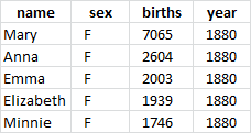
We can read the 1st row as “We had 7065 baby girls named Mary born in the year 1880” and so on…

Moving to Step #2, what was it again? oh yeah, Group the dataframe in Step #1 by name. So let’s do that:

name_gp = all_names.groupby('name');

Yes, it is that easy in the amazing SQL-like Pandas. So now regardless of the Sex and Year columns, group by the name.

The resultant object is of type DataFrameGroupBy, which is not easily accessible as DataFrame object. If you don’t believe me, try to view the first few groups by typing:

name_gp[:5]
#output: TypeError: unhashable type

I will not dive in the cause behind this error, but you may want to know that DataFrameGroupBy objects are of different nature than DataFrame objects, so do not deal with them as they are the same thing. Otherwise, you might get a quite disturbing errors while scratching your head. You might also want to know that many of DataFrameGroupBy object methods such as (apply, aggregate, filter, first, head, last, transform) return a DataFrame object.

Now we get to Step #3, Exclude name groups with records less than 50. As I mentioned above when I enumerated the analysis roadmap, I am doing this Step to extract the common names only, if you like to get ALL unisex names even with few occurrences, skip this Step. So you don’t get shocked if you get different results than mine, remember that the results of this analysis will be presented with this Step included. Here is the code to exclude uncommon names:

names = name_gp.filter(lambda x: len(x) >= 50)

Moving to Step #4, we need to pivot the data to convert the values of the Sex columns (which are M and F) into new columns with the values of births column being aggregated (summed). Need to remind you of table pivot?

names_df = pd.pivot_table(names, values='births', index='name', columns='sex', fill_value=0, aggfunc=sum)

names_df.columns = ['F', 'M']

names_df.reset_index(drop=False, inplace=True)

Notice that in this pivot operation, we sacrificed the year column information, so the summed births values are only related to the name as a key

Why did I suffix this new object with “_gp” because the names within the name column are actually unique, so it feels like we have groups with the name being the key column.

The assignment to columns and resetting the index are just for setting our DataFrame’s headers properly.

Step #5 tells us to Copy the (F, M) columns from the dataframe in the Step #4 into a new dataframe, and here is the code to do it:

tempDF = names_df[['M','F']].copy()

We made this copy to prepare for normalization in Step #6 which is Normalize the columns (F, M) in the copied DataFrame to have the proportion of both genders. I need to emphasise a note here, if you try to normalize them in the same dataframe, the values of columns (M, F) will be overridden. Here is the explanation behind it, we need to keep the absolute values of M, F columns, my reason is that I want to sum them to get an idea about how common a name is compared to other names later. Here is the code to normalize the values within the copied version of the DataFrame:

tempDF = tempDF.div(tempDF.sum(axis=1), axis=0)

This is an efficient use of the methods div and sum, lets divide and conquer to understand it, the code

tempDF.sum(axis=1)

Returns a Pandas.Series object with the sum of the rows of tempDF. which means gets the sum of (F, M) births for every name in the dataframe. Then in the code

tempDF = tempDF.div(tempDF.sum(axis=1), axis=0)

We divide each and every value of tempDF (in both columns F and M) on their corresponding sum (sum of that row, no summing over columns is done here). In the end, we assign the resultant dataframe back to tempDF itself. So for example, if we have a name with 450 boys and 300 gils, we end up with a proportional M value of:

and a proportional F value of:

Of course, the proportional values of M and F are (and should always be) equal to 1. Otherwise, you have something wrong with your normalization code.

Now in Step #7, we need to return the proportional values of M and F to the original dataframe from which we copied them. BUT, we should give them new names so we don’t override their original values:

names_df['Fprop'] = tempDF['F']

names_df['Mprop'] = tempDF['M']

let’s get a view of how we are doing now, shall we?

names_df[:5]

Here is the result:

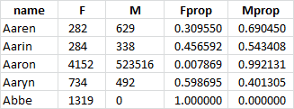
Hmmm… Interesting. We are getting to it, bear with me…

Next, in Step #8 we need to create a new column total_births in which we sum both of M and F columns for every row in the dataframe.

names_df['total_births'] = names_df['M'] + names_df['F']

I’ve added this new column because I want to exclude names with less than 8,000 births, we have data for about 130 years, if a name doesn’t achieve 8,000 births at least, then it is not common, that’s what Step #9 is for. If you want to get ALL unisex names even with only 300 births over 131 years so skip this step.

names_df = names_df[names_df['total_births'] >= 8000]

Moving to Step #10 which is to subset the DataFrame we got from Step #9. This subsetting as mentioned above keeps only those rows with Female proportion between 0.3333 and 0.6666. Notice that we could have done the same thing with Male gender, it doesn’t matter since we only care about the middle third. Here is the final line of code in this analysis:

unisex = names_df[(names_df['Fprop'] >= 0.3333) & (names_df['Fprop'] <= 0.6666)]

Now we have the unisex names in unisex DataFrame.

At first, I wrote this article with sorting the dataframe by the new column total_births descendingly. This was so we get a list of unisex names arranged by popularity. But then I found a better approach, so I will add a new step to the analysis roadmap above:

11. Create a metric derived from the ratio of girls to boys, to indicate how close that name is to be divided equally between both genders, sort by this new metric.

Here is how you do it:

unisex['distance'] = np.abs(unisex['Fprop'] - 0.5)

That means you take the value of Fprop the proportion of girls, subtract 0.5 from it and convert the result into an absolute value, that will get you a value where the closer it is to 0, the closer for its name to be equally divided between genders, that’s why I call this new metric “distance”. We don’t care about which unisex names are used more for girls or boys, we need unisex names, and that’s what we have.

What is left is to sort by our metric distance ascendingly.

unisex = unisex.sort(columns='distance', ascending=True)

Now we have the final list of unisex names, notice that this list is not specific for a decade or this year, but it is for all the data we have (from 1880 to 2010).

unisex[:20]

Voilà! We have the top 20 unisex names

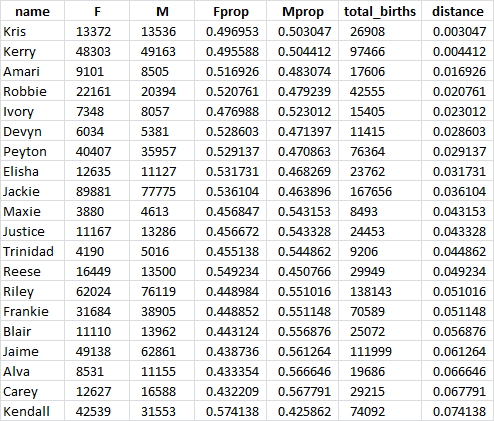
Notice that these unisex names such as Kris and Kerry are not the most common unisex names by popularity but they are the closest names to be equally divided among boys and girls, that’s why they top the list.

Plotting Names

For us to make sure that our analysis is correct, it would be both fun and beneficial to plot some names from the unisex names list. Keep in mind that we cannot plot the names from the unisex dataframe as it doesn’t have the births per year data but we have already used it to know the names of interest to plot, so we can plot them from a different dataframe:

name_year_gp = pd.pivot_table(names, values='births', index=['name', 'year'], columns='sex', fill_value=0, aggfunc=sum)

name_year_gp.columns = ['F', 'M']

name_year_gp.reset_index(drop=False, inplace=True)

Notice that in this dataframe we kept the yearly births. This is a compatible dataframe from which we can plot.

let’s plot the 1st unisex name “Kris”:

plotName(name_year_gp, 'Kris')
# you can find the code of the function plotName below

Here is the resultant plot:

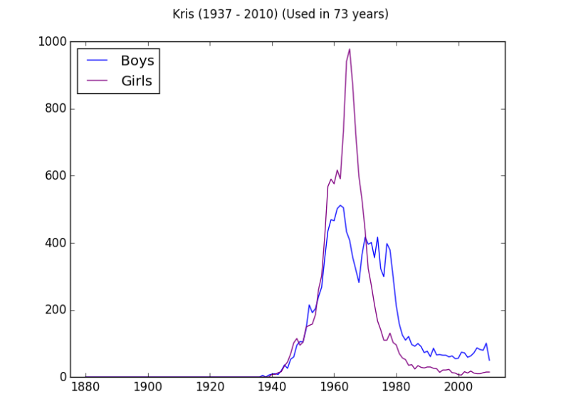
Interesting huh? The name Kris has witnessed a fierce competition between boys and girls over the years, only then to drop for both.

Here is the code of the function plotName used above:

def plotName(df, vName):
    from matplotlib import pyplot as plt

    min_year = df[df['name']==vName]['year'].min()
    max_year = df[df['name']==vName]['year'].max()
    name_used = df[df['name']==vName]['year'].count()

    x = range(1880, 2011)

    m = pd.Series(index = x, data = 0)

    m[df[df['name'] == vName]['year']] = df[df['name'] == vName]['M'].values

    f = pd.Series(index = x, data = 0)

    f[df[df['name'] == vName]['year']] = df[df['name'] == vName]['F'].values

    x = np.array(x)

    plt.plot(m.index, m.values, color='blue')

    plt.plot(f.index, f.values, color='purple')

    plt.xlim(1875, 2015)

    plt.suptitle("{} ({} - {}) (Used in {} years)".format(vName, min_year, max_year, name_used))

    plt.legend(["Boys", "Girls"], loc="upper left")

    plt.show()

Here are other four unisex names, I encourage you to plot some other uni-sex names of your choice.

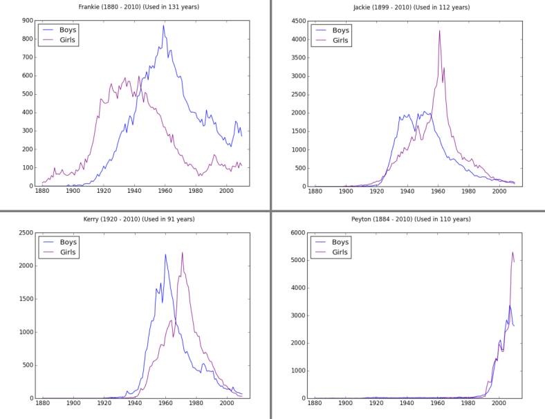
As you can see, obviously, these names are unisex. Data do not lie…

Conclusion

If you enjoyed this data analysis use case, I would be very grateful if you would help it spread by emailing it to a friend, or sharing it on Twitter or Facebook. Thank you!

Keep an eye for the next post, an advanced data analysis where I will give you a good challenge to improve your data analysis skills.

Life is Random But Not Fair – The Difference Between Random vs. Probabilistic Experiments

Introduction

You might remember from your high school math class that the mathematical notation for the probability of an event C is:

And that the probability is the long-term relative frequency of occurrence of some event. That relative frequency is always within the range [0, 1]. That makes complete sense, since it is a ratio, a fraction where the numerator is either less or equal but never greater than the denominator. If you run into an event whose probability is 1, that event is definitely certain, on the other hand, an event whose probability is 0 is impossible. A probability of an event could take any decimal value between 0 and 1 (such as 0.129643, 0.33333, 0.9…etc.).

Probabilistic Experiment

Probabilistic is a very general term and it means there is uncertainty in the process where the outcomes of some event may or may not have fair (equal) probability of occurring. I notice that with more complex examples in nature/real-life, the fancy term “stochastic” is used.

Probabilistic Experiment Example

Let’s say we have this experiment where we throw two fair dice, and we are interested in the sum of the observed top faces of the dice.

Let’s define two events:

Event A: getting a sum which is greater than 4.

Event B: getting a sum which is less or equal to 4.

These two events are compound events. A compound event is an event which has more than one outcome. The events which have only one outcome are called simple events.

The outcome of a fair dice is a random variable, this random variable’s probability distribution is the uniform distribution as the die is fair. From the definition of uniform distribution, we can deduce the following:

If an experiment has a uniform distribution, the probability of an event (either simple or compound) is the number of possible outcomes divided by the total number of possible outcomes.

But, although the sum of two fair dice is another random variable, its probability distribution is not uniform.

Check Figure 1, these are all the possible outcomes in our sample space which is usually called S

Figure 1 – Two Dice Experiment Possible Outcomes

Event B outcomes are the yellow annotated pairs (Figure 2) which sums are all less than or equal to 4 and the total possible outcomes are )

Figure 2 – Event B Possible Outcomes

Therefore, probability of event B is:

And since events A and B are mutually exclusive which means they can’t happen at the same time, the probability of either A or B occurring is:

And since our two events take up all the sample space S, we have

So the probability of event A:

Of course, we could have calculated the probability of event A, the same way we did with event B:

Voila! there we have a probabilistic experiment with two events, with unequal probabilities, the individual outcomes are random (they have equal probabilities) as the dice are fair dice, but the events we defined are not random and one of them (event A) is more likely to happen. We can say that this experiment is biased to event A.

Figure 3 – Events Outcomes

Figure 4 – Events Probabilities

Random Experiment

Random experiment is a special case of probabilistic experiment where all the events in an experiment have (fair) equal probabilities of happening. Ironically enough, except for life which we think of as random but we all agree it is NOT fair!

Example: Drawing one card out of a standard 52-card deck gives 1/52 probability for each of the cards (given no preference or prior information whatsoever about any of the cards, as opposed to the probabilistic experiment I explained above, we don’t want any bias here as we are assuming full randomness).

Finally, I believe that a random experiment is a special case of probabilistic experiment, that case where all the events in the experiment have equal probabilities.

Measures of Central Tendency – The Median

To continue on our roadmap in measures of central tendency, I am about to explain another measure of central tendency, the median.

The median and the mean are both very important measures of central tendency but each has its own properties, let’s start with defining what the median is, then a comparison between the two measures will be made in the next post.

The Median

You might have read this news or this one where the term “median” was used. Without prior knowledge of the term “median”, I suppose that the message by the news item is not really delivered to the reader, is it? This shows the need for news websites to present some statistical concepts when they convey some descriptive news (away from the breaking terrifying ones!).

The median is the value found at the center of values of a random variable, when (and only when) those values are in order (ascending or descending, both works but stick with ascending as it makes more sense and will ease the concept of “quantiles” which I will present later).

Let’s start with a simple example, here is a dummy random variable:

17, 29, 15, 19, 1, 7, 86

First, we need to order these values in an ascending order:

1, 7, 15, 17, 19, 29, 86

Then we select the value in the middle (where the count of the values to its left is equal to the count of values to its right), so obviously the value (17) is the median of this variable, where three values (1, 7, 15) are to its left and three values (19, 29, 86) are to its right.

If we try to generalize this methodology to make it like an algorithm to find the median of a random variable, we start by ordering the values in an ascending order, then we count the values, if the count is an odd number, then we simply select the value in the middle. Otherwise, if the count is an even number, we select the middle two numbers and calculate their arithmetic mean.

I will use the variable temperature from our tiny dataset as an example to explain how you find/calculate the median of a random variable for the case when the values count is an even number.

Let’s first list the values of the variable temp:

14.2, 16.4, 11.9, 15.2, 18.5, 22.1, 19.4, 25.1, 23.4, 18.1, 22.6, 17.2

First, we need to order these values in ascending order:

11.9, 14.2, 15.2, 16.4, 17.2, 18.1, 18.5, 19.4, 22.1, 22.6, 23.4, 25.1

Now, count the values… right we have 12 values which is an even number, so we need to calculate the mean of the middle two values (18.1, 18.5) and we will get the median of our random variable temp which is 18.3

Note: If the count of values is an odd number, then the median is necessarily equal to one of the values. Otherwise, if the count of the values in your random variable is an even number, then the median may or may not be equal to one or more values of that variable (I will leave it as an exercise for you to tell when the median of a random variable with an even number of values is equal to one or more of its values).

As you can see, it is extremely easy and straightforward to find/calculate the median of a random variable. However, you might be faced with some random variables with hundreds, thousands or even millions of observations (values), will you waste days to count them? Fortunately enough, all statistical software packages provide a way to calculate the median of a random variable. Here I will show you how you can calculate the median in Excel and in R.

Calculate Median in Excel

In Excel, you can use the function median to calculate the median of some values, just provide the cells range (Figure1) and Excel will provide you with their median value.

Figure 1 – Excel Median Function

Then press Enter to let Excel know that we finished typing our function, you will get the median value (Figure 2)

Figure 2: Excel – Median Value

Calculate Median in R

In R, you can use the function median to calculate the median of some values, below I provide the necessary R code to calculate the median, applying it on the same variable temp:

temp <- c(14.2, 16.4, 11.9, 15.2, 18.5, 22.1, 19.4, 25.1, 23.4, 18.1, 22.6, 17.2)

median(temp)

#R will print

[1] 18.3

Notice that the median value given by R which is (18.3), is the same value given earlier by Excel, and that makes sense as the method behind calculating the median is the same in all statistical software packages.

Notice also that we didn’t have to present the values in order (either in Excel or in R). However, the statistical software packages managed to calculate the right median value.

The importance of any measure of central tendency like the median, comes from its ability to summarize the whole variable with a single value and it is one way of telling the “central location” of a variable. In this sense, the median is the halfway value in any random variable as we can say that 50% of the values are greater than the median and 50% of the values are less.