Measures of Central Tendency – The Median

To continue on our roadmap in measures of central tendency, I am about to explain another measure of central tendency, the median.

The median and the mean are both very important measures of central tendency but each has its own properties, let’s start with defining what the median is, then a comparison between the two measures will be made in the next post.

The Median

You might have read this news or this one where the term “median” was used. Without prior knowledge of the term “median”, I suppose that the message by the news item is not really delivered to the reader, is it? This shows the need for news websites to present some statistical concepts when they convey some descriptive news (away from the breaking terrifying ones!).

The median is the value found at the center of values of a random variable, when (and only when) those values are in order (ascending or descending, both works but stick with ascending as it makes more sense and will ease the concept of “quantiles” which I will present later).

Let’s start with a simple example, here is a dummy random variable:

17, 29, 15, 19, 1, 7, 86

First, we need to order these values in an ascending order:

1, 7, 15, 17, 19, 29, 86

Then we select the value in the middle (where the count of the values to its left is equal to the count of values to its right), so obviously the value (17) is the median of this variable, where three values (1, 7, 15) are to its left and three values (19, 29, 86) are to its right.

If we try to generalize this methodology to make it like an algorithm to find the median of a random variable, we start by ordering the values in an ascending order, then we count the values, if the count is an odd number, then we simply select the value in the middle. Otherwise, if the count is an even number, we select the middle two numbers and calculate their arithmetic mean.

I will use the variable temperature from our tiny dataset as an example to explain how you find/calculate the median of a random variable for the case when the values count is an even number.

Let’s first list the values of the variable temp:

14.2, 16.4, 11.9, 15.2, 18.5, 22.1, 19.4, 25.1, 23.4, 18.1, 22.6, 17.2

First, we need to order these values in ascending order:

11.9, 14.2, 15.2, 16.4, 17.2, 18.1, 18.5, 19.4, 22.1, 22.6, 23.4, 25.1

Now, count the values… right we have 12 values which is an even number, so we need to calculate the mean of the middle two values (18.1, 18.5) and we will get the median of our random variable temp which is 18.3

Note: If the count of values is an odd number, then the median is necessarily equal to one of the values. Otherwise, if the count of the values in your random variable is an even number, then the median may or may not be equal to one or more values of that variable (I will leave it as an exercise for you to tell when the median of a random variable with an even number of values is equal to one or more of its values).

As you can see, it is extremely easy and straightforward to find/calculate the median of a random variable. However, you might be faced with some random variables with hundreds, thousands or even millions of observations (values), will you waste days to count them? Fortunately enough, all statistical software packages provide a way to calculate the median of a random variable. Here I will show you how you can calculate the median in Excel and in R.

Calculate Median in Excel

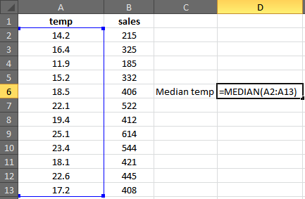
In Excel, you can use the function median to calculate the median of some values, just provide the cells range (Figure1) and Excel will provide you with their median value.

Figure 1 – Excel Median Function

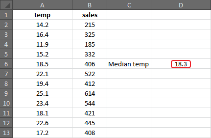
Then press Enter to let Excel know that we finished typing our function, you will get the median value (Figure 2)

Figure 2: Excel – Median Value

Calculate Median in R

In R, you can use the function median to calculate the median of some values, below I provide the necessary R code to calculate the median, applying it on the same variable temp:

temp <- c(14.2, 16.4, 11.9, 15.2, 18.5, 22.1, 19.4, 25.1, 23.4, 18.1, 22.6, 17.2)

median(temp)

#R will print

[1] 18.3

Notice that the median value given by R which is (18.3), is the same value given earlier by Excel, and that makes sense as the method behind calculating the median is the same in all statistical software packages.

Notice also that we didn’t have to present the values in order (either in Excel or in R). However, the statistical software packages managed to calculate the right median value.

The importance of any measure of central tendency like the median, comes from its ability to summarize the whole variable with a single value and it is one way of telling the “central location” of a variable. In this sense, the median is the halfway value in any random variable as we can say that 50% of the values are greater than the median and 50% of the values are less.

Measures of Central Tendency

Measures of central tendency are measures which define the central tendency of observations of some random variable. These measures try to describe a quantitative random variable by summarizing it in single valued numbers. What’s more clear than that? Measures of Central Tendency:

• Mean
• Median
• Mode

I will explain each in a separate post but I want to give you a heads-up. The mean and the median are two different measures of the central tendency of a data variable and sometimes they give two very different ideas about the same variable, especially when the variable contains outliers (extremely low or extremely high values).

If you have the seeds to be a professional data analyst, you would throw that bold sentence in my face and say “This doesn’t tell me anything!”. I know that might be uncalled for but you could be that angry and you are right about that, because there must be a formal way of defining when a value is extremely high or extremely low and the good news is that there is. Bare with me until we get literate enough to explore that new area.

Descriptive Statistics of a Variable – Roadmap

In Dissecting a Dataset, we showed the elements of a dataset from an eagle’s eye. In the simple dataset we used there, it is easy to examine a variable of the dataset by viewing it in Excel or any spreadsheet software or even a text editor. This is because we had only 12 observations in that dataset and only 2 variables; But what to do when we have thousands (or millions?) of observations? Clearly, viewing the data by visualizing it in a spreadsheet is not a feasible option, as one gets lost in the numbers and detecting a pattern in this case is hard, especially if the data comes from a real life process which turns out to be highly volatile and prone to be affected by many many factors.

Due to what is mentioned above, and also sometimes the need to tell something about your data to someone without giving them all the data, came the need to find a formal and exact way to describe data variables and so, some measures have been defined for this very matter.

First I will give a general idea about the measures of central tendency of a random variable, namely, the mean, median and mode, then I will dedicate a post for each of them in this list:

• Mean (the arithmetic average).
• Median.
• Mode.

Then I will go further to describe the measure of dispersion of a random variable:

• Range and Interquartile Range (IQR).
• Variance.
• Standard Deviation.

Then I will discuss how the measures of central tendency change in relation to each other, and how they affect and are affected by the measures of dispersion. Stay tuned!